Getting Started with IceFrame: A Beginner’s Guide to Apache Iceberg’s newest Python Library

Need a free Iceberg Catalog to try with Iceframe, sign up for Dremio’s free 30-day Trial
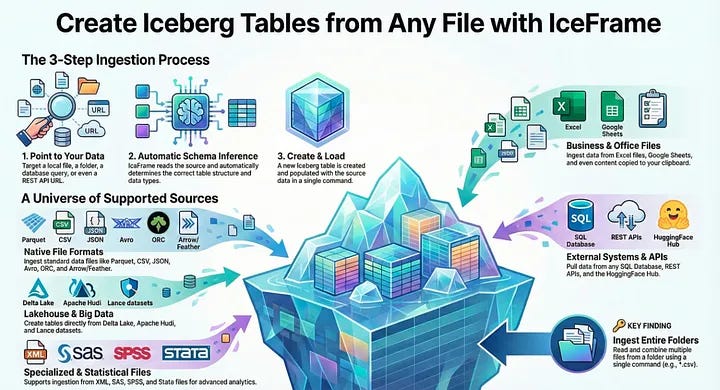
Organizations are increasingly turning to the data lakehouse architecture to manage and analyze their vast datasets. At the heart of this modern architecture is Apache Iceberg, an open table format that brings the reliability and performance of data warehouses directly to data lakes. While Iceberg is incredibly powerful, interacting with it can sometimes feel complex.
Enter IceFrame, a user-friendly and powerful Python library designed to simplify every aspect of working with Iceberg tables. Whether you’re a data engineer building robust pipelines or a data scientist exploring new datasets, IceFrame provides an intuitive, Pythonic interface to get the job done.
This article is your hands-on, step-by-step guide to getting started with IceFrame. We’ll walk you through the core operations, from initial configuration and table creation to querying, writing data, and managing your tables. Let’s dive in and unlock the power of your Iceberg lakehouse with Python!
1. Setup and Configuration: Connecting to Your Catalog
Getting connected with IceFrame is straightforward and is handled primarily through environment variables. This approach keeps your credentials and configuration details separate from your code, which is a security best practice.
The essential variables needed to connect to a standard REST catalog are listed below.
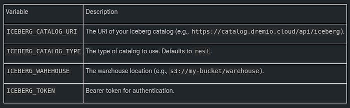
You can place these variables in a .env file in your project’s root directory for IceFrame to automatically load them.
Example .env file:
ICEBERG_CATALOG_URI=https://catalog.example.com
ICEBERG_TOKEN=your-catalog-token
ICEBERG_WAREHOUSE=s3://my-datalake/warehouse
With the environment variables set, initializing the IceFrame client in your Python script is as simple as this:
from iceframe import IceFrame
from iceframe.utils import load_catalog_config_from_env

# Load configuration from environment variables
config = load_catalog_config_from_env()
# Initialize the IceFrame client
ice = IceFrame(config)
2. Creating Your First Iceberg Table
IceFrame makes table creation incredibly simple and supports multiple schema formats to fit your needs. For beginners, the most direct method is to define the schema using a Python dictionary.
The following code demonstrates how to create a new table named products. The schema is defined by mapping column names as keys to their corresponding Iceberg data types as values.
# Define schema using a Python dictionary
schema = {
    “id”: “long”,
    “name”: “string”,
    “price”: “double”,
    “active”: “boolean”,
    “created_at”: “timestamp”,
    “birth_date”: “date”
}

# Create the table in the default namespace
ice.create_table(”products”, schema)
While using a dictionary is great for getting started, IceFrame also supports defining schemas from PyArrow schema objects and Polars DataFrames, offering more control and flexibility for advanced use cases.
3. Writing Data to Your Table
Once your table is created, you’ll want to add data to it. IceFrame provides two primary methods for this: appending new data or overwriting existing data.
Appending Data
Appending is a common operation that adds new rows to a table without affecting existing records. The append_to_table method is perfect for this. Let’s create a Polars DataFrame with data for our products table, ensuring the data types align with the schema we defined earlier (id as a 64-bit integer for long, price as a float for double, etc.).
import polars as pl
from datetime import datetime, date

# Create a Polars DataFrame with new product data
new_products = pl.DataFrame({
    “id”: [101, 102],
    “name”: [”Eco-Friendly Water Bottle”, “Wireless Charging Pad”],
    “price”: [19.99, 25.50],
    “active”: [True, True],
    “created_at”: [datetime(2023, 10, 26, 10, 0, 0), datetime(2023, 10, 26, 10, 5, 0)],
    “birth_date”: [date(2023, 1, 1), date(2023, 1, 5)] # Using date object for date type
})
# Append the DataFrame to the ‘products’ table
ice.append_to_table(”products”, new_products)
Overwriting Data
The overwrite_table method is used when you need to replace the contents of a table completely. This is useful for scenarios like daily reporting, where each day’s data replaces the previous day’s snapshot.
Note: It is crucial to ensure that the data types in your DataFrame match the table’s schema exactly. For instance, a column defined as long in Iceberg expects an int64 data type from Polars or Pandas.
4. Reading and Querying Data
IceFrame provides a flexible and efficient API for reading data from your Iceberg tables, complete with performance-enhancing features like column selection and predicate pushdown.
Simple Reads
To fetch all data from a table into a Polars DataFrame, simply use the read_table method.
# Read the entire ‘products’ table into a Polars DataFrame
df = ice.read_table(”products”)
print(df)
Selective Reads
For better performance, especially on wide tables, you should only select the columns you actually need. You can do this by passing a list of column names to the columns parameter. This reduces the amount of data that needs to be read from storage and transferred over the network.
# Read only the ‘name’ and ‘price’ columns
df_selective = ice.read_table(”products”, columns=[”name”, “price”])
Filtering Data
Just as selecting specific columns reduces data transfer, filtering rows at the source is even more powerful. This technique, called predicate pushdown, ensures that only the data you need is ever read from storage, dramatically speeding up queries on large tables. IceFrame leverages this powerful Iceberg feature by allowing you to provide a SQL-like filter expression to the filter_expr argument.
# Read products that are active and cost more than $20
df_filtered = ice.read_table(”products”, filter_expr=”price > 20.00 AND active = true”)
Time Travel
Apache Iceberg’s time travel capability allows you to query the state of a table as it existed at a previous point in time. IceFrame exposes this feature by allowing you to specify a snapshot_id.
# Read the table as it existed at a specific snapshot
df_historical = ice.read_table(”products”, snapshot_id=123456789012345)
5. Ingesting Data from External Files
A common data engineering task is creating Iceberg tables from existing data files like CSV or Parquet. IceFrame includes convenient methods to handle this with a single line of code.
Here are a couple of examples showing how to create tables from popular file formats.
Creating a table from a Parquet file:
# Schema is inferred directly from the Parquet file
ice.create_table_from_parquet(”my_namespace.table_from_parquet”, “data.parquet”)
Creating a table from a CSV file:
# Schema is inferred from the CSV content
ice.create_table_from_csv(”my_namespace.table_from_csv”, “data.csv”)
IceFrame supports a wide range of other file formats, including JSON, Avro, and ORC, through optional dependencies. For a full list, be sure to check the official documentation.
6. Evolving Your Table Schema
One of the standout features of Apache Iceberg is its support for safe schema evolution. You can add, drop, or rename columns without rewriting the entire table, a massive advantage for large datasets. IceFrame provides a simple alter_table interface to perform these operations.
Let’s see how to perform a common evolution task: adding a new column to our products table.
# Add a new ‘stock_quantity’ column to the ‘products’ table
ice.alter_table(”products”).add_column(”stock_quantity”, “int”, doc=”Number of units in stock”)
Other supported operations include drop_column and rename_column, making it easy to adapt your tables as your data requirements change over time.
7. A Glimpse into Advanced Features
IceFrame is more than just a CRUD interface for Iceberg; it’s a comprehensive toolkit. As you grow more comfortable, here are a few advanced features you might want to explore:
• Table Maintenance: Over time, tables with many small updates can suffer from the “small file problem,” which degrades query performance. IceFrame provides simple maintenance procedures like compact_data_files to optimize your tables by combining small files into larger, more efficient ones.
• Branching & Tagging: For advanced data management and quality workflows, IceFrame supports Iceberg’s branching and tagging capabilities. Branching allows you to create isolated versions of your tables for experimentation or to implement data quality patterns like Write-Audit-Publish (WAP), ensuring that consumers only see validated data.
• AI Agent: IceFrame includes a built-in AI Agent that turns natural language into action. You can ask questions like ‘Show me active products older than 30 days,’ and the agent will generate the correct IceFrame Python code to retrieve that data, helping you explore schemas, discover data, and get performance tips.
Conclusion
In this guide, we’ve covered the fundamentals of getting started with IceFrame. You’ve learned how to configure your connection, perform essential CRUD operations, run powerful queries, evolve your table schema, and even peeked at some of the library’s advanced capabilities. With its simple, Pythonic interface, IceFrame provides a comprehensive toolkit for building and managing a high-performance data lakehouse on Apache Iceberg.
Now that you have the basics, what data challenges will you solve with your Iceberg lakehouse?